

What Expected Goals Explained Means for Modern Football
xG is a football statistic that measures the quality of a chance. It tells you how likely a player is to score from a particular shot, using a scale from 0 to 1. A shot with an xG of 0.2 means a player would score that chance 20% of the time. A penalty has a fixed xG value of 0.76. The metric was invented in 2012 by Opta’s Sam Green and is now a standard part of football analytics.
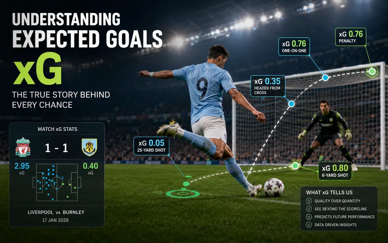
- A long-range shot from 25 yards often has an xG of around 0.02 to 0.05
- A close-range header from a cross can have an xG of 0.3 to 0.5
- A one-on-one with the goalkeeper usually has an xG of about 0.76
- A penalty has a fixed xG of 0.76
- A shot from six yards out can have an xG as high as 0.8
Why Scorelines Alone Mislead Match Analysis
The final score does not always tell the full story. A 1-1 draw can hide a completely one-sided performance. Liverpool vs Burnley match on January 17, 2026. Game ended 1-1. Liverpool had 2.95 xG. Burnley had only 0.4 xG. Liverpool created enough chances to win comfortably, but they did not convert them. The scoreline made it look like a fair result. The xG told a very different story.
How xG Calculates Shot Quality From Real Data
The xG model is built on data from nearly one million historical shots. Advanced machine learning analyses over 20 variables. These include distance from goal, angle, defensive pressure, and goalkeeper location. The model then calculates the percentage chance. This gives the probability that a player would score from that position and situation.
| Shot Type | Typical xG Value | What It Means |
| 25-yard shot | 0.05 | Would be scored 5% of the time |
| 18-yard shot | 0.10 | Would be scored 10% of the time |
| Header from cross | 0.35 | Would be scored 35% of the time |
| One-on-one | 0.76 | Would be scored 76% of the time |
| Penalty | 0.76 | Would be scored 76% of the time |
Key Variables That Shape Every Shot Probability
Many factors affect a shot’s xG value. Distance from goal is the most important factor. The angle of the shot also matters. A shot from a tight angle is harder to score than one from the centre of the box. The type of shot changes the probability. Number of defenders between shooter and goal also impact xG value. Goalkeeper position matter too. All these factors are considered in the xG model.
Reading Match Reports Using Expected Goals Explained
xG is not about predicting the result of a single match. It is a tool for understanding performance over time. A team can dominate the xG battle and still lose. But over 10 or more matches, xG gives a reliable picture of a team’s attacking quality and defensive solidity.
- Overperforming: A team scores more goals than their xG suggests.
- Underperforming: A team scores fewer goals than their xG suggests.
When Teams Outperform Their xG Numbers
Some teams consistently score more than their xG suggests. This is often because they have world-class finishers. Erling Haaland is the best example. He actually scored nearly three more goals than expected. That is a differential of +2.86. Clinical finishers like Haaland can turn half-chances into goals. So when a team overperforms their xG. Then it usually comes down to the quality of their strikers.
When xG Predicts Future Performance Better Than Goals
xG is a better predictor of future performance than actual goals. Goals can be random. They can be influenced by luck. Over a full season, the xG table often gives a more accurate picture. The 2025-26 Premier League xG table showed interesting results. Several teams performed different from real league position. West Ham were relegated from the Premier League. But they conceded five goals more than they should have based on xG.
Real Match Examples That Prove xG Value
Liverpool vs Burnley match on January 17, 2026, is perfect case study. Liverpool had 2.95 xG. Burnley had only 0.56 xG. The match ended 1-1. The xG numbers showed that Liverpool created far better chances. They had 32 shots. Had 11 on target. And 76 touches in the opposition box. Burnley had only one goal from a rare counter-attack. The xG explained why the result felt so frustrating for Liverpool fans.
Case Study: Liverpool vs Burnley 2025-26 Season
Liverpool had 32 shots in the match. Burnley had only a handful. Liverpool’s xG of 2.95 meant they were expected to score nearly three goals. They only scored one. Burnley’s xG of 0.4 meant they were expected to score less than one goal. The 1-1 draw was a classic example of a team failing to convert their chances. The xG data showed that Liverpool dominated the game. The scoreline did not.
How xG Reveals Hidden Dominance in Close Games
Close scorelines can hide dominant performance. Crystal Palace had 4.30 xG against Bournemouth in the 2025-26 Premier League. That is an extraordinary number for a single game. It means Palace created enough chances to score four goals. The actual score might have been much tighter. xG helps understand which teams truly controlled a match.
Using xG Guide to Evaluate Player Performance
xG is not just for teams. It is also used to evaluate individual players. It removes penalties from the calculation. This gives a clearer picture of a player’s open-play finishing ability.
Strikers Who Consistently Beat Their xG
Erling Haaland is the most reliable overperformer in world football. His average xG per shot in the 2025-26 season was 0.27. That is much higher than the 0.17 xG per shot. Higher than what he had at the start of the previous season. It means the chances he got in 2025-26 were easier to score. But he still scored more than expected. They need more chances to score the same number of goals.
Midfielders Creating High xG Chances Without Scoring
xG is also used to evaluate creative players. xA measures the quality of chances a player creates. It looks at chances created for teammates. A midfielder who makes progressive passes will have high xA numbers. A midfielder who plays through balls will also have high xA numbers. This is true even if they do not score goals themselves. Bruno Fernandes often create high-quality chances. Bruno Fernandes had an xG of 1.8 from open play. That means he created chances worth nearly two goals. He did this without scoring himself.
Common xG Mistakes Fans and Pundits Make
xG is a powerful tool, but it is often misunderstood. Many fans and pundits make basic errors when using it.
Why One Match xG Does Not Tell the Full Story
xG is not designed for single matches. One game can produce misleading numbers. A team can have a high xG and still lose. A team can have a low xG and still win. The predictive power of xG comes from larger sample sizes. It takes about 10 matches for xG to start telling a reliable story.
Conclusion
xG is a game-changer for football analysis. It is because it measures the quality of chances. It does not just count the number of shots. It gives context to results. It helps fans understand why a 1-1 draw can feel like a loss for one team. It can also feel like a win for the other team. xG also helps predict future performance. Teams that consistently create high-quality chances usually start scoring more goals.
The metric has practical uses for clubs too. Liverpool signed Mohamed Salah in 2017. Their analysts preferred his xG values. They chose him over other targets. That decision changed the club’s history. xG is not perfect. It does not account for the quality of the specific player taking the shot. But it is one of the best tools available for understanding football. Used correctly, it reveals patterns that the scoreboard hides.
Want to understand football with deeper insights and expert analysis? Follow Sports Arena for the latest football news, tactical breakdowns, match analysis, and exclusive sports stories delivered every day.
